Building a Bacterial Genome Without Writing Code
Never written a line of code? That is fine. This post is about the biology and the pipeline: why whole-genome sequencing answers questions PCR cannot, what assembly and annotation mean, and how nf-core/bacass turns raw FASTQ into a finished genome. The pipeline runs on the Omicslab platform — if you have not run an nf-core pipeline there before, start with the companion guide How to Run nf-core Pipelines on the Omicslab Platform.
1. First: what is the point of rebuilding a genome?
Imagine you are writing a thesis about an antibiotic-resistant bacterial strain. You need to answer two questions: which antibiotics does it resist, and why does it resist them — so you can explain the mechanism and suggest what to do about it.
The fastest test, PCR, cannot help you here.
1.1. Why PCR is not enough
PCR works on a "know it first, then look for it" principle. To run a PCR, you must already know the sequence you are looking for in order to design a primer. In other words:
- PCR only detects what you already know: a familiar resistance gene, a mutation already described in the literature.
- If the bacterium resists through a novel mechanism — a gene never seen before, a new mutation, or an unfamiliar plasmid — you have no primer to probe with, and PCR returns a misleading negative result.
That is when you need to read the whole genome instead of probing a single spot. You do not have to know in advance what to look for, because all the information is already there in the sequence data.
1.2. What is genome assembly?
A sequencing machine cannot read a whole chromosome in one go. It returns millions of reads — short fragments of sequence (Illumina data) or long ones (Oxford Nanopore, PacBio) — like a book torn into millions of tiny slips of paper, each slip with its text overlapping the slips next to it.
Genome assembly is the job of finding those overlaps and piecing the slips back into a continuous text. The result is an almost complete genome: every gene, mutation and plasmid in the strain — including things nobody has seen before. Then annotation labels the genome, so you know which stretches are genes, what proteins they encode, and what mechanism lies behind the resistance.
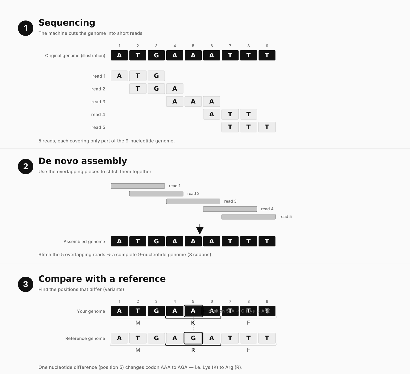
Illustrated with a 9-nucleotide genome (3 amino acids): sequencing, de novo assembly, then comparison against a reference — one nucleotide change alters an amino acid.
There are three biological stages:
- Sequencing — the machine reads the DNA and cuts it into millions of short fragments called reads. Each read is a very short stretch, not enough on its own to conclude anything.
- De novo assembly — using the overlapping pieces between reads to stitch them into continuous stretches (contigs). This step does not need to know what the genome looks like in advance, so it can reveal regions that never appeared in any database.
- Comparison against a reference genome — lining your genome up against a known genome of the same species to find the positions that differ (variants such as SNPs), and to confirm the species. It is the quick way to answer "where does this strain differ from the reference?". If a differing position falls inside a gene, it can change the amino acid — in the figure, a single nucleotide at position 5 turns Lys (K) into Arg (R).
The key point for the PCR story above: comparison against a reference only finds differences from what is already known. A completely new gene will not be in the reference — so we need de novo assembly followed by annotation to find it.
| Term | In plain words |
|---|---|
| Read | One fragment of sequence the machine produced |
| Coverage | How many times, on average, each position in the genome was read — higher is safer |
| Contig | A continuous stretch of assembled sequence |
| N50 | A number describing how long the contigs are; a larger N50 means a more contiguous assembly |
| Short-read | Short, accurate, cheap reads (e.g. Illumina) |
| Long-read | Long reads that bridge repeated regions (e.g. Nanopore, PacBio) |
| Hybrid | Using both short and long reads for the best result |
| Annotation | Labelling the genome: where the genes are and what they do |
A bacterial genome is small — usually just 2–8 million base pairs and often a single circular chromosome. That makes bacterial assembly far easier than the human genome, and an ideal place to start.
2. nf-core/bacass: the box that is already assembled
nf-core/bacass is a shared community pipeline for bacterial genome assembly and annotation.
2.1. What stages does the pipeline run?
It takes raw data (FASTQ) and automatically runs every step you need: quality control, trimming, assembly, contamination screening, assembly quality assessment and annotation.
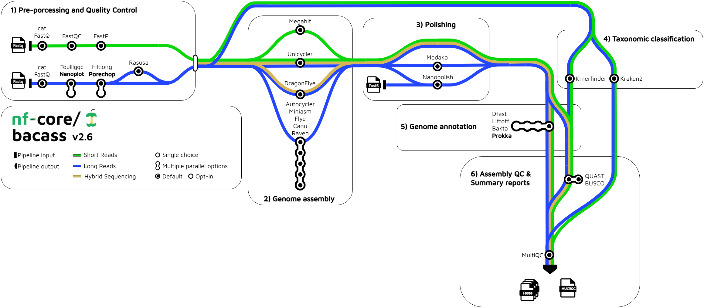
Source: nf-core/bacass (metromap), MIT licence.
On the metromap above, the whole journey looks like a metro line with stations:
| Stage | What runs automatically |
|---|---|
| QC & trimming | FastQC, FastP for short reads; NanoPlot/PycoQC, PoreChop/Filtlong for long reads |
| Assembly | Unicycler, MEGAHIT (short); Flye, Canu, Raven, Miniasm, Dragonflye, Autocycler (long) |
| Contamination screening | Kraken2 and Kmerfinder confirm the sample is not mixed with another species |
| Assembly QC | QUAST and BUSCO — how good the assembly is |
| Annotation | Prokka, Bakta or DFAST — labelling genes and their functions |
Each stage can be switched on or off with a simple parameter, so you never run steps you do not need.
2.2. Three kinds of data: short, long, hybrid
The pipeline supports three kinds of data:
- Short-read — short reads only (Illumina).
- Long-read — long reads only (Nanopore/PacBio).
- Hybrid — both together, for the most contiguous assembly.
3. Preparing your input data
bacass needs a samplesheet: a simple table (TSV, tab-separated) saying which files belong to each sample.
3.1. What columns does the samplesheet have?
Six columns:
| Column | Meaning |
|---|---|
ID |
Sample name, no spaces |
R1, R2 |
Forward and reverse short reads; use NA if absent |
LongFastQ |
Long reads; use NA if absent |
Fast5 |
Fast5 folder (only if polishing the assembly); usually NA |
GenomeSize |
Estimated genome size, e.g. 2.8m for 2.8 million base pairs |
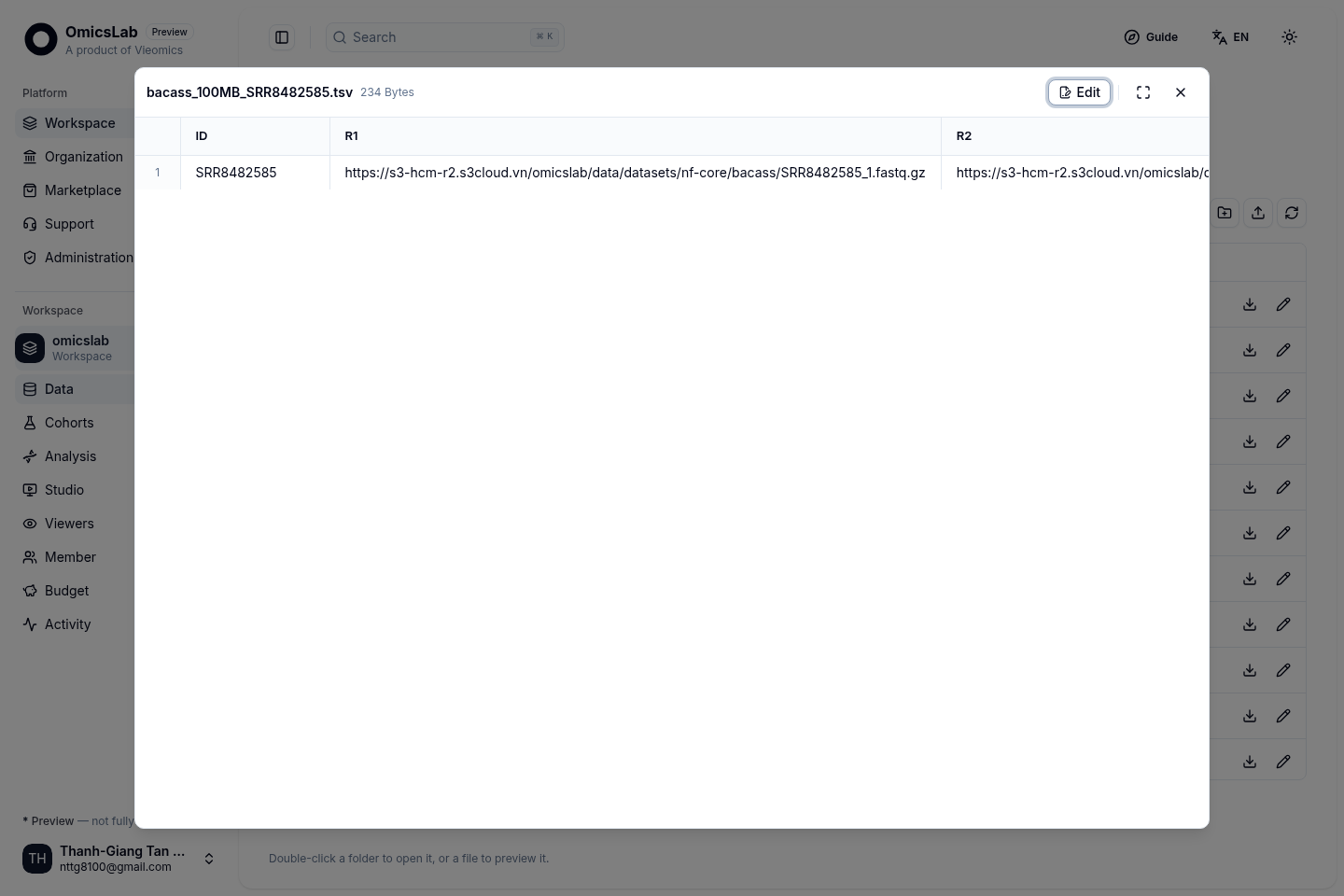
A real samplesheet already available in the omicslab workspace — double-click the .tsv to read it: each row is one sample, with R1/R2 pointing at the FASTQ files.
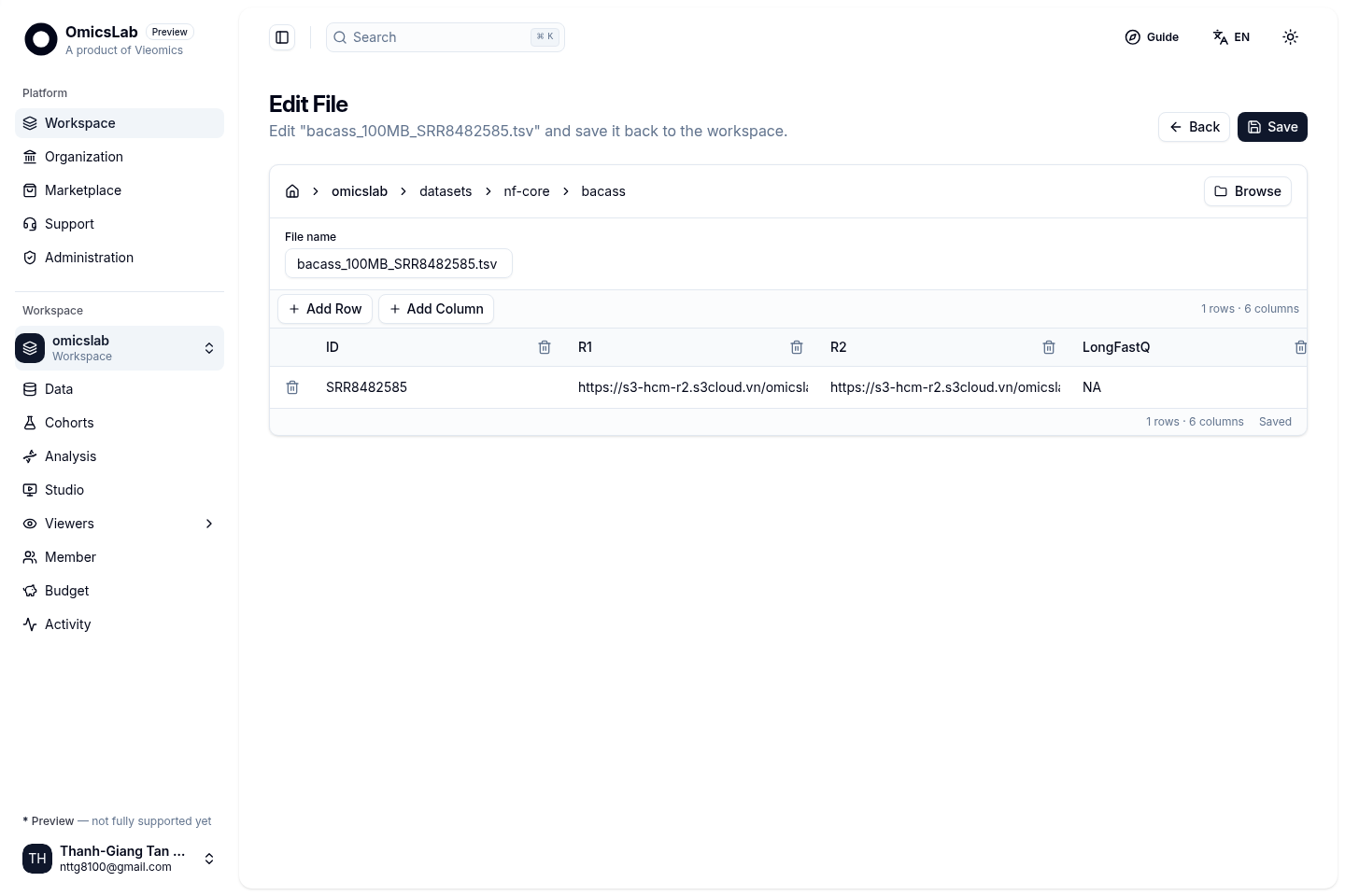
Need to adjust it? Press Edit to open the spreadsheet right on the platform — add rows, add columns and save straight back to the workspace.
3.2. An example samplesheet
An example samplesheet covering all three data types:
| ID | R1 | R2 | LongFastQ | Fast5 | GenomeSize |
|---|---|---|---|---|---|
shortreads |
./data/S1_R1.fastq.gz |
./data/S1_R2.fastq.gz |
NA | NA | NA |
longreads |
NA | NA | ./data/S1_long_fastq.gz |
NA | 2.8m |
shortNlong |
./data/S1_R1.fastq.gz |
./data/S1_R2.fastq.gz |
./data/S1_long_fastq.gz |
NA | 2.8m |
No data yet? The next section shows how to download nf-core's free sample dataset and try the pipeline first.
4. Running nf-core/bacass on the platform
The companion post How to Run nf-core Pipelines on the Omicslab Platform covers the mechanics step by step — creating a workspace, uploading data, adding the pipeline, watching logs and costs. What is specific to bacass is the input and the choices below.
Start with nf-core's free test data. nf-core provides a small bacterial dataset for this pipeline:
- Sample samplesheet: bacass_short_reseq.tsv
- Full sample data repository: nf-core/test-datasets › bacass
Upload the samplesheet and the FASTQ files it references, then choose:
| Parameter | What to pick on a first run |
|---|---|
input |
The samplesheet you uploaded |
assembly_type |
short for Illumina data, long for Nanopore/PacBio, hybrid for both |
assembler |
unicycler (short reads), flye (long reads), dragonflye (hybrid) — or another assembler the pipeline supports |
annotation_tool |
prokka (fast, classic), bakta or dfast |
busco_lineage |
bacteria_odb10 (the default) |
kraken2db |
Needed only if you keep contamination screening on |
skip_kraken2, skip_kmerfinder |
Turn on for the very first test run; turn them back on once you are familiar |
Press Run, watch the Nextflow log stream in the browser, and open the job from History when it finishes. The 100 MB sample dataset used for the screenshots finished in about 30 minutes for 13,318 VND.
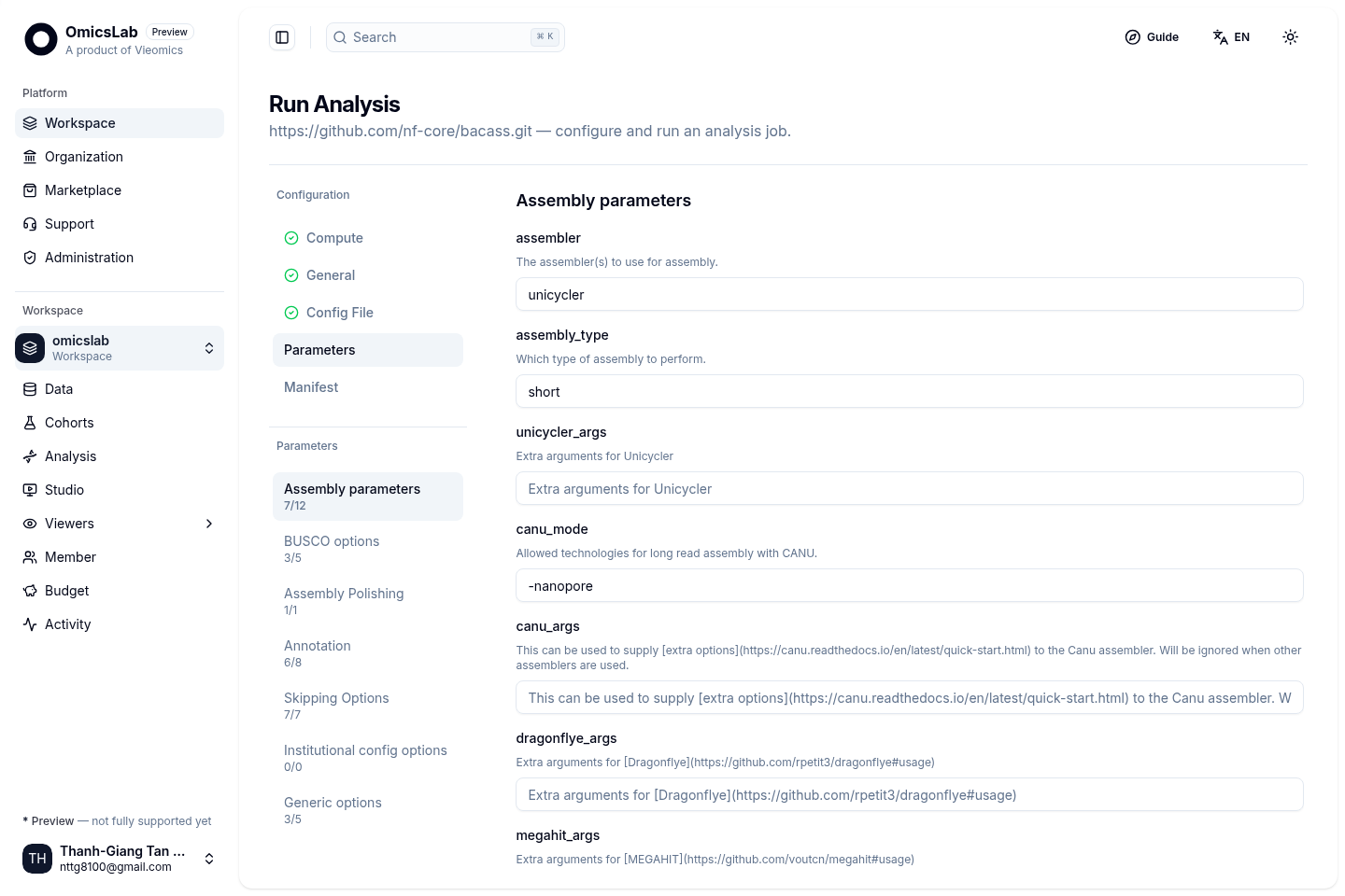
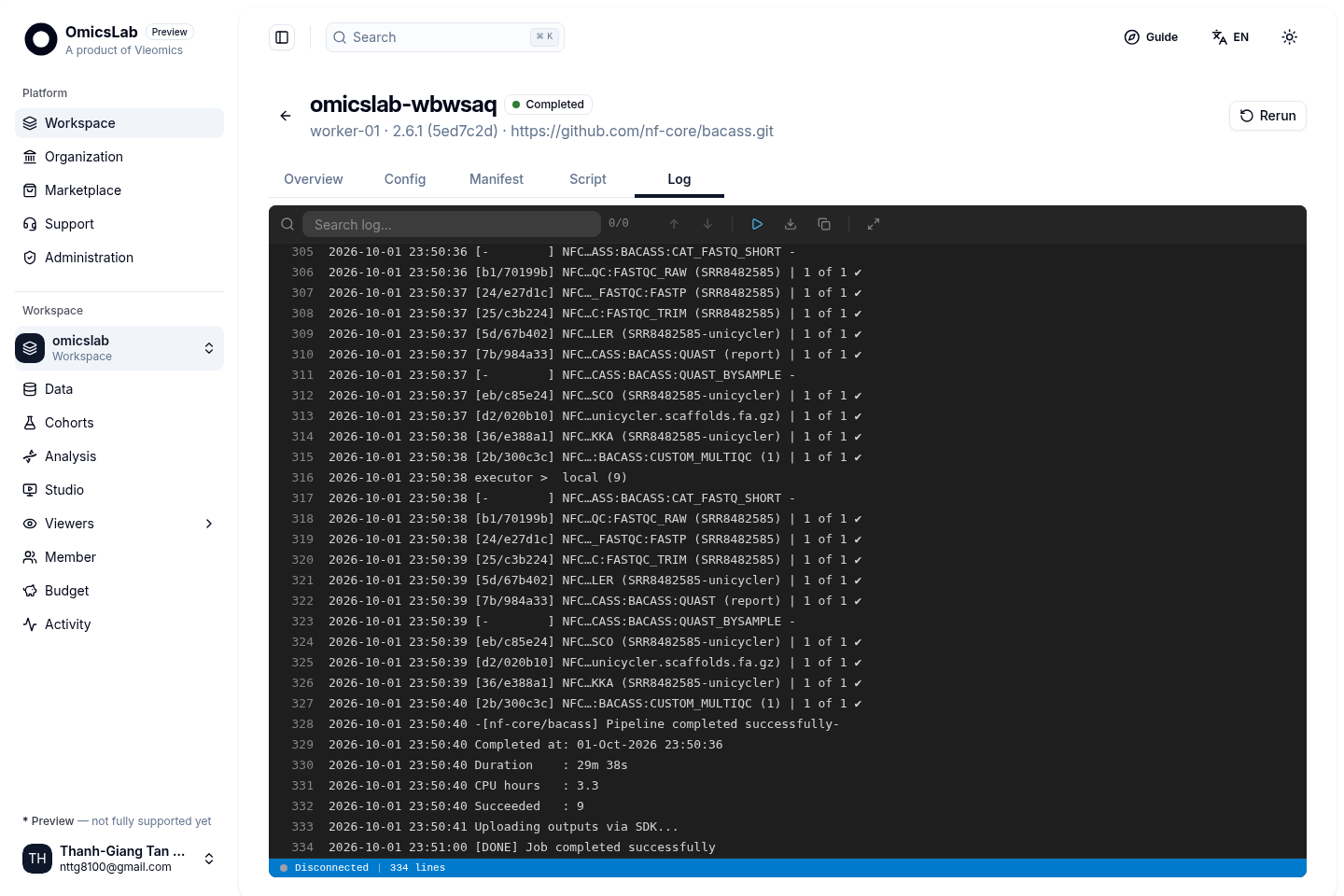
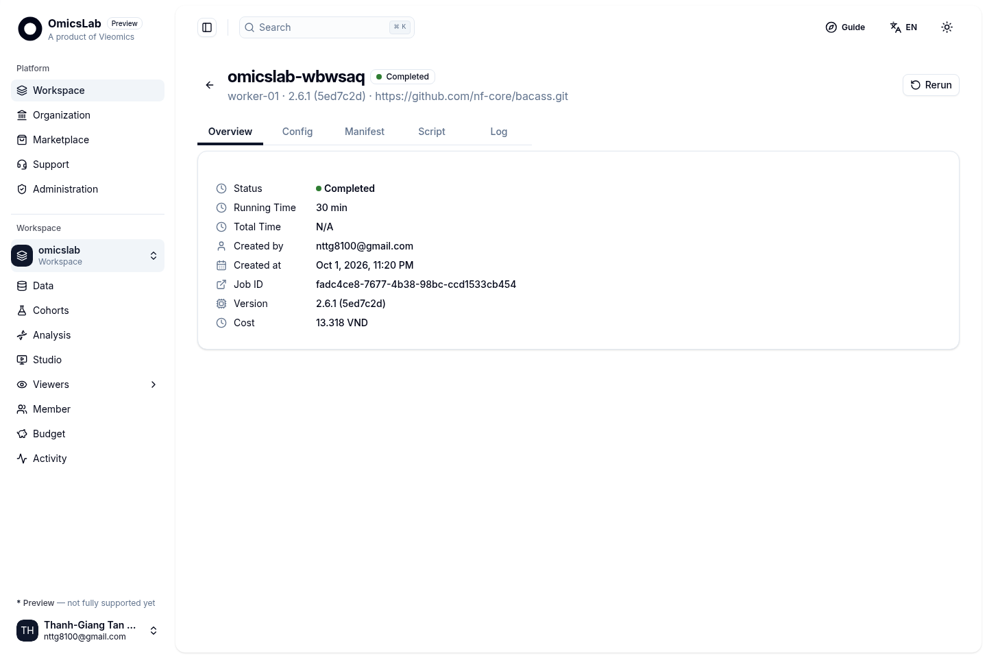
For your first run, use a single sample with nf-core's sample dataset. Once it works, add more samples to the same samplesheet — the platform will run them in parallel.
5. Reading the results
When the pipeline finishes, you get one tidy results folder:
| Output | What it tells you |
|---|---|
*_assembly.fasta |
The assembled genome sequence |
| QUAST report | Contig count, N50, total length — assembly quality |
| BUSCO report | Share of essential genes found — completeness |
| Kraken2 / Kmerfinder report | Whether the sample is contaminated by another species |
Annotation files (.gff, .gbk) |
Gene locations and predicted functions |
| MultiQC report | One page summarising every other report |
6. A real case study from Vietnam
6.1. The melioidosis study in Ha Tinh
To see how far this pipeline can go, look at a real study. In 2026, a Vietnamese and international research team published in PLOS Neglected Tropical Diseases the sequencing of 47 Burkholderia pseudomallei strains — the bacterium that causes melioidosis. The strains were collected at Ha Tinh Provincial General Hospital in 2020, together with soil samples and two animal samples.
The notable part: they assembled the genomes with exactly the nf-core/bacass workflow this post walks through — FastP trimming, Unicycler assembly, Prokka annotation — before going further.
6.2. Results and the lesson
From the assembled genomes, the team:
- Typed the strains with MLST and cgMLST (matching gene sequences against public databases).
- Built a whole-genome SNP phylogeny to trace transmission and compare against nearly 1,500 other strains from Southeast Asia and Australia.
- Found a gene region specific to the dominant strain group (ST 41) and proposed it as a new diagnostic target.
The headline result: 60% of cases belonged to a single strain (ST 41), and those strains were closely linked to soil samples from the same area — pointing to an environment-to-human transmission route.
The lesson: this is exactly the kind of question PCR struggles with. Nobody knew the "ST 41 gene region" existed in advance to design a primer — it only surfaced once the whole genome was read.
Norris MH, Au La TH, Metrailer MC, et al. (2026). Expanding the molecular epidemiology of melioidosis in North Central Vietnam. PLOS Neglected Tropical Diseases, 20(2), e0013945. doi.org/10.1371/journal.pntd.0013945
All data from the study is public at NCBI SRA under PRJNA1180080.
7. Open ending: your turn
There are two ways to start right now:
- Re-run it on this very dataset. Download the FASTQ files from SRA under
PRJNA1180080(or use nf-core's sample data), upload them to the platform and run nf-core/bacass following the platform guide. You will walk the same path the research team did — and you can verify the result yourself. - Explore deeper tools on the platform. Once you have a genome, you can find and add other pipelines from their Git repositories — as long as they provide a run script and a parameter schema. A few directions:
- Species identification and comparison against reference strains.
- MLST / cgMLST to type the strain.
- Whole-genome SNP analysis and phylogenetic trees for epidemiology.
- Pan-genome analysis to find genes specific to a strain group.
- Submit the data to a public database (e.g. NCBI) to share it.
There is no single correct pipeline for every question. Try things, compare them, and work out what fits — the platform does not lock you into one fixed toolset.
Got a result or a question? Share it with us at contact@omicslab.io.
8. Get started
- Create an account at platform.omicslab.io — no credit card required.
- Create a workspace and add the
nf-core/bacasspipeline. - Try it with nf-core's sample data, then swap in your own.
- Need help or a fully managed run? Write to contact@omicslab.io.
9. References
- nf-core/bacass — documentation, parameters and example results: nf-co.re/bacass
- Platform docs — Quickstart, Organizations and Marketplace
- Case study — Norris MH, et al. (2026), Expanding the molecular epidemiology of melioidosis in North Central Vietnam, PLOS Neglected Tropical Diseases 20(2): e0013945. doi.org/10.1371/journal.pntd.0013945
- Public data — NCBI SRA BioProject PRJNA1180080
10. Related Articles
- Platform guide: How to Run nf-core Pipelines on the Omicslab Platform.
- More posts on bioinformatics and pipelines.
- Features and pricing on the Omicslab Platform page.
- Need a fully managed service? See Custom Solutions.
- Official pipeline documentation: nf-co.re/bacass.