Part 3 of 5 — How can a country build its own 1000 Genomes Project? Variant calling, cohort analytics, and data organization
In Part 1 and Part 2, we covered the architecture, design principles, and the implementation roadmap. This part starts with variant calling and joint genotyping, then goes deep into the Hail cohort analytics layer and the storage architecture.
Series Overview
- Part 1: Vision and end-to-end architecture
- Part 2: Design principles and implementation roadmap
- Part 3 (This Post): Variant calling, cohort analytics, and data organization
- Part 4: Infrastructure, talent, and government support: 2018 → 2026
- Part 5: Summary, extensions, and the questions ahead
1. Variant Calling & Joint Genotyping
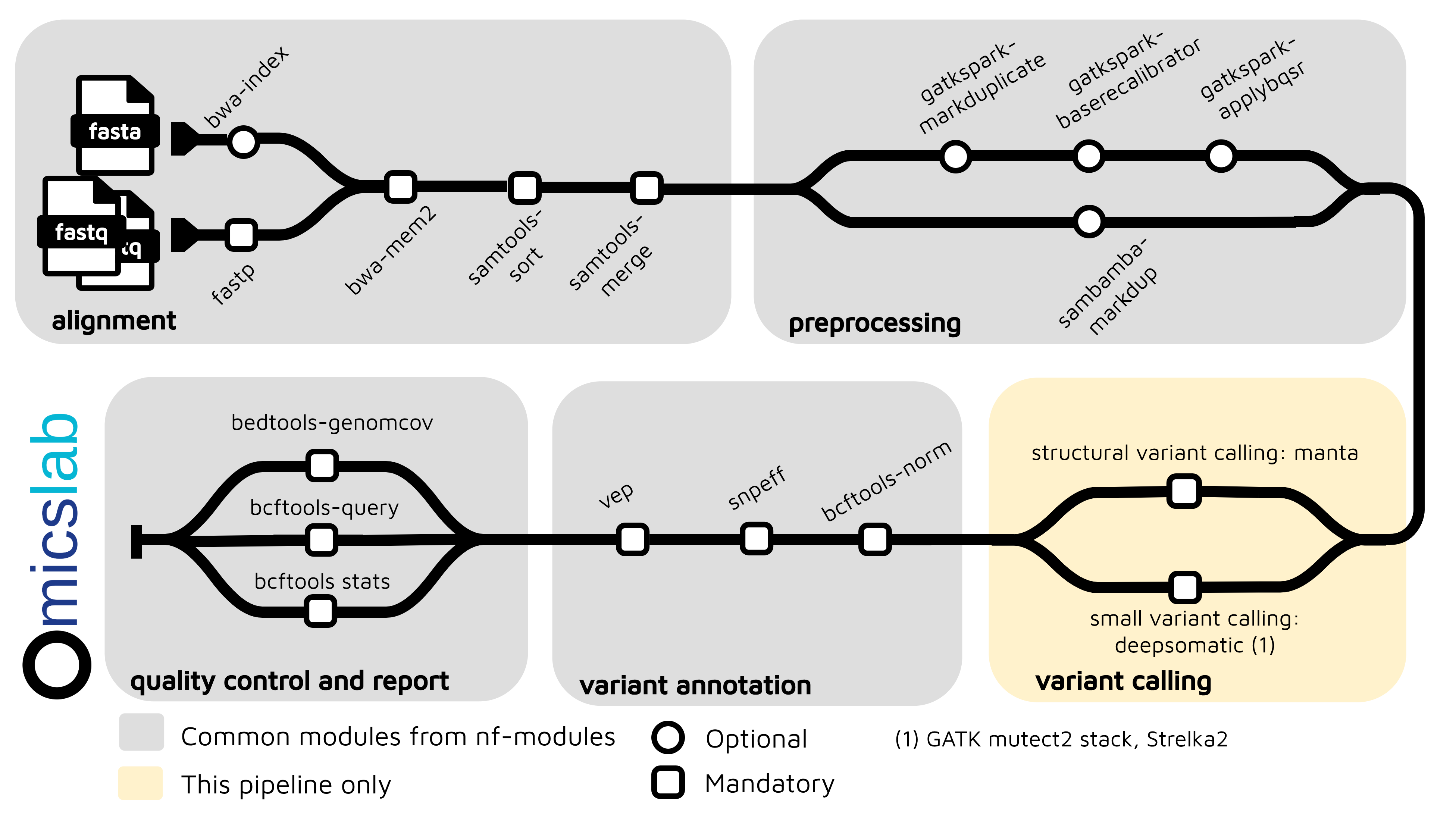
Detailed implementation guides for variant calling and joint genotyping are covered in our dedicated blog series:
- Variant Calling: See our comprehensive series on nf-germline-short-read-variant-calling pipeline
- Joint Genotyping: Detailed technical walkthroughs for GLnexus and DPGT implementations
- Benchmarking: Performance comparisons and optimization techniques
This series focuses on the architecture-level decisions and ecosystem integration rather than pipeline internals. Refer to the dedicated blogs for implementation details, code walkthroughs, and troubleshooting.
2. Cohort Analytics Layer (Hail) — Enabling "Open Work" for Researchers
- The exported data can support multiple research purposes, including integration with EHR and external datasets.
- The following sections are for illustration only; practical analyses typically require more extensive effort.
2.1. Why the Analytics Layer Matters
The true value of a national genome project emerges in the "open work" phase—when researchers can freely query your 1k-sample cohort to answer scientific questions. This requires more than just storing raw genotypes. You need:
- Multiple export formats (PLINK, BGEN, VDS) so different research tools can work efficiently
- Population statistics (allele frequencies, ancestry information, phenotype summaries) accessible to all researchers
- Quality-controlled, analysis-ready data that researchers can trust
- Fast query infrastructure (MatrixTable, HailQL) for exploratory analysis
The analytics layer is the difference between "we have genome data" and "researchers can use our genome data."
This section shows how to build that infrastructure.
2.2. From Raw VCF to Research-Ready Data
Once you have a cohort VCF with all samples jointly-called, the next critical step is transforming it into analysis-ready formats and populating metadata for QC and filtering.
Why Hail for this layer:
- Scalable: Processes cohort VCFs with 100k+ samples efficiently
- Flexible: Export to PLINK, BGEN, VDS, or keep as MatrixTable
- Production-ready: Used by major biobanks (UK Biobank, gnomAD, etc.)
- Analytics integration: Built-in for GWAS, burden tests, population statistics
2.3. Hail MatrixTable Workflow
Load cohort VCF:
import hail as hl
# Import cohort VCF into Hail MatrixTablemt = hl.import_vcf('s3://genome-project/cohort.vcf.gz')
# MatrixTable structure:# - Rows: Variants (SNPs, indels, etc.)# - Columns: Samples# - Entries: Genotypes (0/0, 0/1, 1/1, ./.)Add annotations:
# Variant-level annotationsmt = hl.vep(mt) # Functional predictionmt = mt.annotate_rows( gnomad_af = gnomad.rows()[mt.row_key].AF, clinvar_sig = clinvar.rows()[mt.row_key].significance)
# Sample-level annotations (sex, ancestry, phenotype)mt = mt.annotate_cols( sex = sample_meta[mt.col_key].sex, ancestry = sample_meta[mt.col_key].ancestry, case_status = sample_meta[mt.col_key].phenotype)QC filtering:
# Sample QCsample_qc = hl.sample_qc(vds)mt = mt.annotate_cols(qc = sample_qc[mt.col_key])
# Filter based on QC metricsmt = mt.filter_cols( (mt.qc.n_het > 0) & # Has heterozygous calls (mt.qc.dp_mean > 30) & # Average depth >30x (mt.qc.r_ti_tv > 2.0) # Ti/Tv ratio normal)
# Variant QCmt = mt.filter_rows(hl.agg.count_where(mt.GT.is_non_ref()) > 0)Export to analysis-ready formats:
# PLINK format (for GWAS)hl.export_plink(mt, 'cohort.bed', 'cohort.bim', 'cohort.fam')
# BGEN format (compact, efficient)hl.export_bgen(mt, 'cohort.bgen')
# VDS (Hail native, best for future Hail analyses)mt.write('s3://genome-project/cohort.vds', overwrite=True)2.4. Population-Level Statistics
Calculate allele frequencies:
# Global allele frequenciesmt = mt.annotate_rows( allele_freq = hl.agg.allele_stats(mt.GT).AF, ac = hl.agg.count_where(mt.GT.is_non_ref()), an = hl.agg.count() * 2)
# Ancestry-stratified frequencies (if multi-population)mt = mt.annotate_rows( freq_by_ancestry = hl.agg.collect_as_dict( mt.ancestry, hl.agg.allele_stats(mt.GT).AF ))Population genetics calculations:
# Hardy-Weinberg equilibriummt = mt.annotate_rows( hwe = hl.hardy_weinberg_test( hl.agg.count_where(mt.GT == hl.call(0, 0)), hl.agg.count_where(mt.GT == hl.call(0, 1)), hl.agg.count_where(mt.GT == hl.call(1, 1)) ))
# Principal Component Analysis (population structure)pc_eigenvalues, pc_scores, pc_loadings = hl.pca( mt.GT.n_alt_alleles(), k=20, compute_loadings=True)2.5. Variant Annotation Pipeline
Integrate external resources:
# ClinVar pathogenicityclinvar = hl.read_table('gs://hail-datasets/clinvar.ht')mt = mt.annotate_rows( clinvar_sig = clinvar.rows()[mt.row_key].significance)
# gnomAD frequencies (population reference)gnomad = hl.read_table('gs://hail-datasets/gnomad.ht')mt = mt.annotate_rows( gnomad_ac = gnomad.rows()[mt.row_key].AC, gnomad_af = gnomad.rows()[mt.row_key].AF)
# CADD scores (variant effect prediction)cadd = hl.read_table('path/to/cadd.ht')mt = mt.annotate_rows( cadd_score = cadd.rows()[mt.row_key].score)Create interpretable variant categories:
# Flag likely pathogenic variantsmt = mt.annotate_rows( is_likely_pathogenic = ( (mt.clinvar_sig == 'pathogenic') | ((mt.cadd_score > 30) & (mt.gnomad_af < 0.01)) ), is_rare = mt.gnomad_af < 0.01, is_common = mt.gnomad_af > 0.05)2.6. Rare Disease Interpretation & Diagnosis
Using cohort as background reference:
# For each rare disease sample, find matching variants in cohort# Example: Exome analysis with population context
rare_disease_mt = hl.read_matrix_table('rare_disease_samples.vds')
# Annotate with cohort allele frequenciesrare_disease_mt = rare_disease_mt.annotate_rows( cohort_af = mt.rows()[rare_disease_mt.row_key].allele_freq, cohort_ac = mt.rows()[rare_disease_mt.row_key].ac)
# Prioritize rare variants (absent or very rare in cohort)rare_disease_mt = rare_disease_mt.filter_rows( (rare_disease_mt.cohort_ac < 5) | # <5 people in cohort hl.is_missing(rare_disease_mt.cohort_af) # Not in cohort at all)2.7. Example Research Projects ("Open Work")
This is where the value of your genome project becomes visible. Once the infrastructure is ready, researchers can immediately begin:
Example 1: Genome-Wide Association Study (GWAS)
# Researcher has 1k individuals, 500 with Type 2 Diabetes, 500 without# Goal: Find variants associated with diabetes in your population
from hail.methods import linear_regression_rows
# Load PLINK formatmt = hl.read_table('cohort.plink')
# Fit linear regression: genotype ~ diabetes statusmt = mt.annotate_rows( beta = linear_regression_rows( y=mt.phenotype.diabetes, x=mt.GT.n_alt_alleles() ))
# Find significant associationsgwas_hits = mt.filter_rows(mt.p_value < 5e-8)
# Result: 50-200 genome-wide significant variants unique to your populationExample 2: Rare Variant Burden Test in Specific Genes
# Researcher: "I think inactivating mutations in Gene X cause Disease Y"# Goal: Test if individuals with mutations in Gene X have higher disease rates
# Filter to rare variants in Gene Xgene_x_variants = mt.filter_rows( (mt.gene == "GENE_X") & (mt.gnomad_af < 0.01) # Rare in world population)
# Count carriers in cases vs. controlscase_carriers = mt.filter_cols(mt.phenotype.is_case).filter_rows( mt.GT.is_non_ref()).count_rows() / mt.count_cols()
# Perform burden test (logistic regression)burden_test = hl.logistic_regression_rows(...)
# Result: "Individuals with rare variants in Gene X are 5x more likely to have Disease Y"Example 3: Population Stratification & Ancestry-Specific Allele Frequencies
# Researcher: "How does allele frequency of SNP rs123 differ by ancestry?"
# PCA on your 1k cohort (calculated in 2.3)mt = mt.annotate_cols( ancestry = predicted_ancestry[mt.col_key] # PC-based ancestry labels)
# Allele frequencies stratified by ancestrymt = mt.annotate_rows( af_by_ancestry = hl.agg.collect_as_dict( mt.ancestry, hl.agg.allele_stats(mt.GT).AF ))
# Result: "SNP rs123 is 10% in European ancestry, 3% in African ancestry"# Clinical implication: Frequency interpretation depends on patient ancestryExample 4: Clinical Variant Interpretation
# Clinician: "I have a patient with a rare variant; how common is it?"# Query your public allele frequency database (built from 2.4)
# Web interface: Enter variant rs123456# System returns: "This variant found in 2 of 1000 samples (0.2%)"# "gnomAD says 0.05%, so it's enriched in your population"# "ClinVar classification: Likely pathogenic"# "VEP prediction: This affects splicing"
# Result: Clinician has population-specific evidence for clinical interpretationExample 5: Longitudinal Health Outcomes (if EHR linked)
# Researcher: "Do people with high polygenic risk scores develop heart disease earlier?"# Requires: 5+ years of follow-up data
# Build PRS from GWAS hitsprs = hl.sum_prs(mt_gwas_hits)
# Predict time-to-disease (Kaplan-Meier curves)survivors_by_prs = mt.annotate_cols( prs = prs, years_to_disease = ehr_data[mt.col_key].years_to_heart_disease)
# Result: "High PRS group: 30% disease by age 60; Low PRS group: 5%"# "This enables risk stratification in your healthcare system"2.8. Monitoring Data Quality & Variant Drift
As years pass, you may want to ensure variant calls remain stable:
# Annual QC check: Re-call a subset of samples with latest pipelinemt_revalidation = hl.import_vcf('revalidated_samples.vcf.gz')
# Compare allele frequencies to historical recordsmt_historical = mt.filter_rows(mt_revalidation.row_key)
# Should be nearly identical (small differences OK, large drift is problem)af_concordance = hl.corr( mt_historical.allele_freq, mt_revalidation.allele_freq)
# Flag if >0.01 drift (suggests pipeline changes or batch effects)if af_concordance < 0.99: alert("Variant frequency drift detected; investigate pipeline changes")3. Storage Architecture & Data Organization
3.1. Three-Tier Storage Strategy
Tier 1: Raw Archive (gVCFs)
s3://genome-project/archive/gvcfs/├── 2026/01/sample_001.gvcf.gz├── 2026/01/sample_002.gvcf.gz...├── 2026/12/sample_12000.gvcf.gz
Purpose: Immutable source data (5-10 year retention)Access: Restricted to data stewardsStorage class: Cold storage (infrequent access)Tier 2: Processed Cohort (VCFs)
s3://genome-project/processed/├── cohort_2026_q1.vcf.gz (Jan-Mar samples)├── cohort_2026_q1.vcf.gz.tbi├── cohort_2026_q2.vcf.gz (Apr-Jun samples)...
Purpose: QC baseline, joint-called sourceAccess: Project researchers with approvalRetention: 5+ yearsStorage class: Standard (frequent access)Tier 3: Analytics Ready
s3://genome-project/analytics/├── cohort_combined.plink.* (PLINK bed/bim/fam)├── cohort_combined.bgen (BGEN format)├── cohort_combined.vds/ (Hail VDS)├── population_stats/ (AF, AC, HWE tables)└── public_release_v3.0/ (Anonymized for sharing)
Purpose: Analysis-ready, indexed, compressedAccess: Researchers, public (stratified by tier)Retention: Indefinite for currentStorage class: Standard3.2. Metadata Organization
Sample metadata:
samples.tsvcol1: sample_idcol2: institutioncol3: sexcol4: ancestrycol5: case_statuscol6: sequencing_datecol7: pipeline_versioncol8: qc_pass (true/false)Variant metadata (stored in VCF header & annotations):
- Pipeline version (nf-germline-short-read-variant-calling v1.2.3)- Reference genome (GRCh38)- Joint genotyping tool (GLnexus v1.5.2)- Annotation version (VEP version 106)- Date processed (2026-03-15)3.3. Data Versioning & Release Strategy
Public data releases:
v1.0 (2026-06): 500 samples, 30M variantsv1.1 (2026-09): 750 samples, 35M variantsv2.0 (2026-12): 1,000 samples, 40M variants (complete 1k cohort)v2.1 (2027-06): 1,000 samples, 40M variants + updated annotationsv3.0 (2028-06): 1,000 samples, 40M variants + multi-omic layers (if extended work pursued)
Each release:- Frozen cohort VCF (immutable)- Allele frequency tables (stratified by ancestry if multi-population)- QC metrics summary (depth, call rates, Hardy-Weinberg stats)- Known issues & caveats- Citation guidance for researchers using the dataIn Part 4, we look at Vietnam's journey from VN1K's start in 2018 to 2026 — infrastructure, talent, and government support for genomics.
References
Series repositories
- omicslab-hpc — Ansible automation to build the SLURM HPC cluster. https://github.com/vieomics/omicslab-hpc
- nf-germline-short-read-variant-calling — standardized short-read germline variant-calling pipeline. https://github.com/vieomics/nf-germline-short-read-variant-calling
- nf-modules — Nextflow modules and subworkflows shared across the series pipelines. https://github.com/vieomics/nf-modules
- omicslab-kit — gkit proof-of-concept implementations (GLnexus, DPGT, Spark-on-SLURM, Hail). https://github.com/vieomics/omicslab-kit
Sources and further reading
- GLnexus — joint genotyping engine that merges per-sample gVCFs into a cohort VCF. https://github.com/dnanexus-rnd/GLnexus
- DPGT — distributed joint genotyping on Spark. https://github.com/BGI-flexlab/DPGT
- Hail — platform for population-scale genetic analysis, used for the cohort analytics layer. https://hail.is/
This is Part 3 of the series. Continue to Part 4 for Vietnam's 2018 → 2026 journey.