
Phần 3/5 — Làm thế nào một quốc gia xây dựng dự án 1000 Genomes của riêng mình? Gọi biến thể, phân tích cohort và tổ chức dữ liệu
Ở Phần 1 và Phần 2, chúng ta đã có kiến trúc tổng thể, các nguyên tắc thiết kế và lộ trình triển khai. Phần này bắt đầu từ gọi biến thể và joint genotyping, rồi đi sâu vào tầng phân tích cohort bằng Hail và cách tổ chức lưu trữ dữ liệu.
Tổng quan chuỗi bài
- Phần 1: Tầm nhìn và kiến trúc tổng thể
- Phần 2: Nguyên tắc thiết kế và lộ trình triển khai
- Phần 3 (bài này): Gọi biến thể, phân tích cohort và tổ chức dữ liệu
- Phần 4: Hạ tầng, nhân lực và hỗ trợ của Chính phủ: 2018 → 2026
- Phần 5: Tóm tắt, mở rộng và những câu hỏi phía trước
1. Gọi biến thể & joint genotyping
Hướng dẫn triển khai chi tiết cho gọi biến thể và joint genotyping được trình bày trong chuỗi bài chuyên đề của chúng tôi:
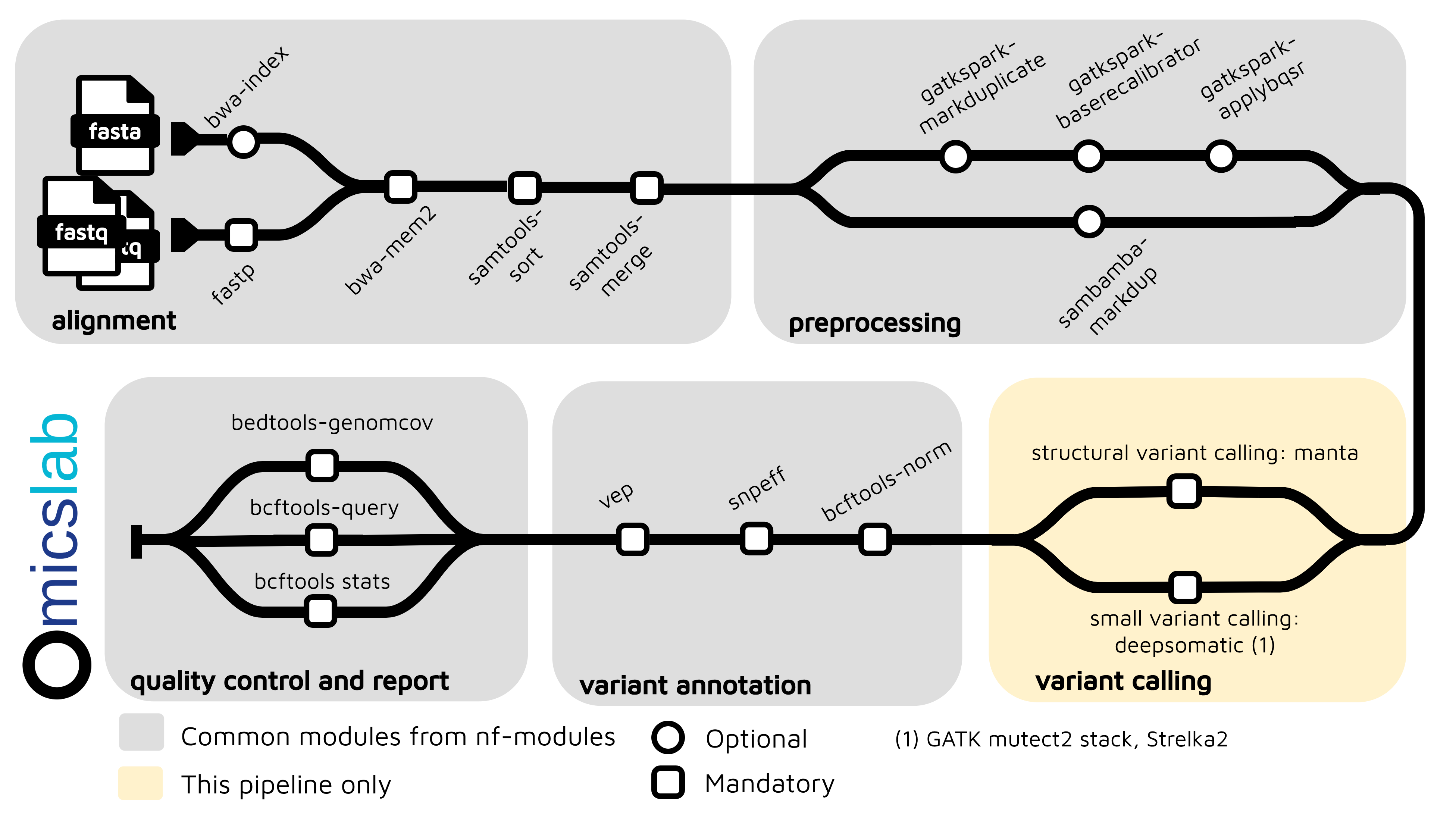
- Gọi biến thể: xem chuỗi bài toàn diện về pipeline nf-germline-short-read-variant-calling
- Joint genotyping: hướng dẫn kỹ thuật chi tiết cho các triển khai GLnexus và DPGT
- Benchmarking: so sánh hiệu năng và kỹ thuật tối ưu hóa
Chuỗi bài này tập trung vào các quyết định ở mức kiến trúc và tích hợp hệ sinh thái thay vì chi tiết nội bộ pipeline. Vui lòng tham khảo các bài chuyên đề để biết chi tiết triển khai, phân tích mã và xử lý sự cố.
2. Tầng phân tích cohort (Hail) — mở đường cho "open work" của nhà nghiên cứu
- Dữ liệu xuất ra có thể hỗ trợ nhiều mục đích nghiên cứu, bao gồm tích hợp với EHR và các bộ dữ liệu bên ngoài.
- Các phần sau chỉ mang tính minh họa; phân tích thực tế thường cần nhiều công sức hơn.
2.1. Vì sao tầng phân tích quan trọng
Giá trị thực sự của một dự án hệ gen quốc gia xuất hiện ở giai đoạn "open work" — khi các nhà nghiên cứu có thể tự do truy vấn cohort 1k mẫu của bạn để trả lời các câu hỏi khoa học. Điều này đòi hỏi nhiều hơn việc chỉ lưu trữ kiểu gen thô. Bạn cần:
- Nhiều định dạng xuất (PLINK, BGEN, VDS) để các công cụ nghiên cứu khác nhau hoạt động hiệu quả
- Thống kê quần thể (tần số allele, thông tin tổ tiên, tóm tắt kiểu hình) mà mọi nhà nghiên cứu đều truy cập được
- Dữ liệu đã kiểm soát chất lượng, sẵn sàng phân tích để nhà nghiên cứu tin tưởng
- Hạ tầng truy vấn nhanh (MatrixTable, HailQL) cho phân tích khám phá
Tầng phân tích là khác biệt giữa "chúng tôi có dữ liệu hệ gen" và "nhà nghiên cứu có thể dùng dữ liệu hệ gen của chúng tôi."
Phần này trình bày cách xây dựng hạ tầng đó.
2.2. Từ VCF thô đến dữ liệu sẵn sàng nghiên cứu
Khi đã có VCF cohort với tất cả mẫu được gọi chung (jointly-called), bước quan trọng tiếp theo là chuyển nó sang các định dạng sẵn sàng phân tích và bổ sung metadata cho QC và lọc.
Vì sao chọn Hail cho tầng này:
- Khả năng mở rộng: xử lý hiệu quả VCF cohort với hơn 100k mẫu
- Linh hoạt: xuất sang PLINK, BGEN, VDS hoặc giữ dưới dạng MatrixTable
- Sẵn sàng production: được các ngân hàng sinh học lớn dùng (UK Biobank, gnomAD, v.v.)
- Tích hợp phân tích: hỗ trợ sẵn cho GWAS, burden test, thống kê quần thể
2.3. Workflow Hail MatrixTable
Nạp VCF cohort:
import hail as hl
# Import cohort VCF into Hail MatrixTablemt = hl.import_vcf('s3://genome-project/cohort.vcf.gz')
# MatrixTable structure:# - Rows: Variants (SNPs, indels, etc.)# - Columns: Samples# - Entries: Genotypes (0/0, 0/1, 1/1, ./.)Thêm chú giải:
# Variant-level annotationsmt = hl.vep(mt) # Functional predictionmt = mt.annotate_rows( gnomad_af = gnomad.rows()[mt.row_key].AF, clinvar_sig = clinvar.rows()[mt.row_key].significance)
# Sample-level annotations (sex, ancestry, phenotype)mt = mt.annotate_cols( sex = sample_meta[mt.col_key].sex, ancestry = sample_meta[mt.col_key].ancestry, case_status = sample_meta[mt.col_key].phenotype)Lọc QC:
# Sample QCsample_qc = hl.sample_qc(vds)mt = mt.annotate_cols(qc = sample_qc[mt.col_key])
# Filter based on QC metricsmt = mt.filter_cols( (mt.qc.n_het > 0) & # Has heterozygous calls (mt.qc.dp_mean > 30) & # Average depth >30x (mt.qc.r_ti_tv > 2.0) # Ti/Tv ratio normal)
# Variant QCmt = mt.filter_rows(hl.agg.count_where(mt.GT.is_non_ref()) > 0)Xuất sang các định dạng sẵn sàng phân tích:
# PLINK format (for GWAS)hl.export_plink(mt, 'cohort.bed', 'cohort.bim', 'cohort.fam')
# BGEN format (compact, efficient)hl.export_bgen(mt, 'cohort.bgen')
# VDS (Hail native, best for future Hail analyses)mt.write('s3://genome-project/cohort.vds', overwrite=True)2.4. Thống kê cấp quần thể
Tính tần số allele:
# Global allele frequenciesmt = mt.annotate_rows( allele_freq = hl.agg.allele_stats(mt.GT).AF, ac = hl.agg.count_where(mt.GT.is_non_ref()), an = hl.agg.count() * 2)
# Ancestry-stratified frequencies (if multi-population)mt = mt.annotate_rows( freq_by_ancestry = hl.agg.collect_as_dict( mt.ancestry, hl.agg.allele_stats(mt.GT).AF ))Các phép tính di truyền quần thể:
# Hardy-Weinberg equilibriummt = mt.annotate_rows( hwe = hl.hardy_weinberg_test( hl.agg.count_where(mt.GT == hl.call(0, 0)), hl.agg.count_where(mt.GT == hl.call(0, 1)), hl.agg.count_where(mt.GT == hl.call(1, 1)) ))
# Principal Component Analysis (population structure)pc_eigenvalues, pc_scores, pc_loadings = hl.pca( mt.GT.n_alt_alleles(), k=20, compute_loadings=True)2.5. Pipeline chú giải biến thể
Tích hợp nguồn dữ liệu bên ngoài:
# ClinVar pathogenicityclinvar = hl.read_table('gs://hail-datasets/clinvar.ht')mt = mt.annotate_rows( clinvar_sig = clinvar.rows()[mt.row_key].significance)
# gnomAD frequencies (population reference)gnomad = hl.read_table('gs://hail-datasets/gnomad.ht')mt = mt.annotate_rows( gnomad_ac = gnomad.rows()[mt.row_key].AC, gnomad_af = gnomad.rows()[mt.row_key].AF)
# CADD scores (variant effect prediction)cadd = hl.read_table('path/to/cadd.ht')mt = mt.annotate_rows( cadd_score = cadd.rows()[mt.row_key].score)Tạo các nhóm biến thể dễ diễn giải:
# Flag likely pathogenic variantsmt = mt.annotate_rows( is_likely_pathogenic = ( (mt.clinvar_sig == 'pathogenic') | ((mt.cadd_score > 30) & (mt.gnomad_af < 0.01)) ), is_rare = mt.gnomad_af < 0.01, is_common = mt.gnomad_af > 0.05)2.6. Giải nghĩa và chẩn đoán bệnh hiếm
Dùng cohort làm tham chiếu nền:
# For each rare disease sample, find matching variants in cohort# Example: Exome analysis with population context
rare_disease_mt = hl.read_matrix_table('rare_disease_samples.vds')
# Annotate with cohort allele frequenciesrare_disease_mt = rare_disease_mt.annotate_rows( cohort_af = mt.rows()[rare_disease_mt.row_key].allele_freq, cohort_ac = mt.rows()[rare_disease_mt.row_key].ac)
# Prioritize rare variants (absent or very rare in cohort)rare_disease_mt = rare_disease_mt.filter_rows( (rare_disease_mt.cohort_ac < 5) | # <5 people in cohort hl.is_missing(rare_disease_mt.cohort_af) # Not in cohort at all)2.7. Các dự án nghiên cứu ví dụ ("open work")
Đây là nơi giá trị của dự án hệ gen trở nên hữu hình. Khi hạ tầng sẵn sàng, nhà nghiên cứu có thể bắt đầu ngay:
Ví dụ 1: Nghiên cứu liên kết toàn hệ gen (GWAS)
# Researcher has 1k individuals, 500 with Type 2 Diabetes, 500 without# Goal: Find variants associated with diabetes in your population
from hail.methods import linear_regression_rows
# Load PLINK formatmt = hl.read_table('cohort.plink')
# Fit linear regression: genotype ~ diabetes statusmt = mt.annotate_rows( beta = linear_regression_rows( y=mt.phenotype.diabetes, x=mt.GT.n_alt_alleles() ))
# Find significant associationsgwas_hits = mt.filter_rows(mt.p_value < 5e-8)
# Result: 50-200 genome-wide significant variants unique to your populationVí dụ 2: Burden test cho biến thể hiếm trong các gene cụ thể
# Researcher: "I think inactivating mutations in Gene X cause Disease Y"# Goal: Test if individuals with mutations in Gene X have higher disease rates
# Filter to rare variants in Gene Xgene_x_variants = mt.filter_rows( (mt.gene == "GENE_X") & (mt.gnomad_af < 0.01) # Rare in world population)
# Count carriers in cases vs. controlscase_carriers = mt.filter_cols(mt.phenotype.is_case).filter_rows( mt.GT.is_non_ref()).count_rows() / mt.count_cols()
# Perform burden test (logistic regression)burden_test = hl.logistic_regression_rows(...)
# Result: "Individuals with rare variants in Gene X are 5x more likely to have Disease Y"Ví dụ 3: Phân tầng quần thể & tần số allele theo tổ tiên
# Researcher: "How does allele frequency of SNP rs123 differ by ancestry?"
# PCA on your 1k cohort (calculated in 2.3)mt = mt.annotate_cols( ancestry = predicted_ancestry[mt.col_key] # PC-based ancestry labels)
# Allele frequencies stratified by ancestrymt = mt.annotate_rows( af_by_ancestry = hl.agg.collect_as_dict( mt.ancestry, hl.agg.allele_stats(mt.GT).AF ))
# Result: "SNP rs123 is 10% in European ancestry, 3% in African ancestry"# Clinical implication: Frequency interpretation depends on patient ancestryVí dụ 4: Giải nghĩa biến thể trong lâm sàng
# Clinician: "I have a patient with a rare variant; how common is it?"# Query your public allele frequency database (built from 2.4)
# Web interface: Enter variant rs123456# System returns: "This variant found in 2 of 1000 samples (0.2%)"# "gnomAD says 0.05%, so it's enriched in your population"# "ClinVar classification: Likely pathogenic"# "VEP prediction: This affects splicing"
# Result: Clinician has population-specific evidence for clinical interpretationVí dụ 5: Kết cục sức khỏe theo thời gian (nếu liên kết EHR)
# Researcher: "Do people with high polygenic risk scores develop heart disease earlier?"# Requires: 5+ years of follow-up data
# Build PRS from GWAS hitsprs = hl.sum_prs(mt_gwas_hits)
# Predict time-to-disease (Kaplan-Meier curves)survivors_by_prs = mt.annotate_cols( prs = prs, years_to_disease = ehr_data[mt.col_key].years_to_heart_disease)
# Result: "High PRS group: 30% disease by age 60; Low PRS group: 5%"# "This enables risk stratification in your healthcare system"2.8. Giám sát chất lượng dữ liệu & biến động biến thể
Qua nhiều năm, bạn có thể muốn đảm bảo các kết quả gọi biến thể vẫn ổn định:
# Annual QC check: Re-call a subset of samples with latest pipelinemt_revalidation = hl.import_vcf('revalidated_samples.vcf.gz')
# Compare allele frequencies to historical recordsmt_historical = mt.filter_rows(mt_revalidation.row_key)
# Should be nearly identical (small differences OK, large drift is problem)af_concordance = hl.corr( mt_historical.allele_freq, mt_revalidation.allele_freq)
# Flag if >0.01 drift (suggests pipeline changes or batch effects)if af_concordance < 0.99: alert("Variant frequency drift detected; investigate pipeline changes")3. Kiến trúc lưu trữ & tổ chức dữ liệu
3.1. Chiến lược lưu trữ ba tầng
Tầng 1: Lưu trữ thô (gVCF)
s3://genome-project/archive/gvcfs/├── 2026/01/sample_001.gvcf.gz├── 2026/01/sample_002.gvcf.gz...├── 2026/12/sample_12000.gvcf.gz
Mục đích: dữ liệu gốc bất biến (lưu trữ 5-10 năm)Truy cập: hạn chế cho bộ phận quản lý dữ liệuLớp lưu trữ: cold storage (truy cập không thường xuyên)Tầng 2: Cohort đã xử lý (VCF)
s3://genome-project/processed/├── cohort_2026_q1.vcf.gz (mẫu tháng 1-3)├── cohort_2026_q1.vcf.gz.tbi├── cohort_2026_q2.vcf.gz (mẫu tháng 4-6)...
Mục đích: chuẩn QC, nguồn đã joint-calledTruy cập: nhà nghiên cứu dự án có phê duyệtThời gian lưu: 5+ nămLớp lưu trữ: standard (truy cập thường xuyên)Tầng 3: Sẵn sàng phân tích
s3://genome-project/analytics/├── cohort_combined.plink.* (PLINK bed/bim/fam)├── cohort_combined.bgen (định dạng BGEN)├── cohort_combined.vds/ (Hail VDS)├── population_stats/ (bảng AF, AC, HWE)└── public_release_v3.0/ (đã ẩn danh để chia sẻ)
Mục đích: sẵn sàng phân tích, có index, nénTruy cập: nhà nghiên cứu, công chúng (phân tầng theo cấp)Thời gian lưu: không thời hạn cho bản hiện tạiLớp lưu trữ: standard3.2. Tổ chức metadata
Metadata mẫu:
samples.tsvcol1: sample_idcol2: institutioncol3: sexcol4: ancestrycol5: case_statuscol6: sequencing_datecol7: pipeline_versioncol8: qc_pass (true/false)Metadata biến thể (lưu trong header VCF & phần chú giải):
- Phiên bản pipeline (nf-germline-short-read-variant-calling v1.2.3)- Hệ gen tham chiếu (GRCh38)- Công cụ joint genotyping (GLnexus v1.5.2)- Phiên bản chú giải (VEP phiên bản 106)- Ngày xử lý (2026-03-15)3.3. Quản lý phiên bản dữ liệu & chiến lược phát hành
Các bản phát hành dữ liệu công khai:
v1.0 (2026-06): 500 mẫu, 30M biến thểv1.1 (2026-09): 750 mẫu, 35M biến thểv2.0 (2026-12): 1.000 mẫu, 40M biến thể (hoàn tất cohort 1k)v2.1 (2027-06): 1.000 mẫu, 40M biến thể + chú giải cập nhậtv3.0 (2028-06): 1.000 mẫu, 40M biến thể + các lớp đa omics (nếu theo đuổi mở rộng)
Mỗi bản phát hành gồm:- VCF cohort đóng băng (bất biến)- Bảng tần số allele (phân tầng theo tổ tiên nếu đa quần thể)- Tóm tắt chỉ số QC (độ sâu, call rate, thống kê Hardy-Weinberg)- Các vấn đề đã biết & lưu ý- Hướng dẫn trích dẫn cho nhà nghiên cứu sử dụng dữ liệuỞ Phần 4, chúng ta nhìn lại hành trình từ khi VN1K khởi động năm 2018 đến năm 2026 — hạ tầng, nhân lực và sự hỗ trợ của Chính phủ cho genomics tại Việt Nam.
Tài liệu tham khảo
Repository của chuỗi bài
- omicslab-hpc — tự động hóa Ansible để dựng cụm SLURM HPC. https://github.com/vieomics/omicslab-hpc
- nf-germline-short-read-variant-calling — pipeline gọi biến thể germline chuẩn hóa từ dữ liệu đọc ngắn. https://github.com/vieomics/nf-germline-short-read-variant-calling
- nf-modules — module và subworkflow Nextflow dùng chung giữa các pipeline trong chuỗi bài. https://github.com/vieomics/nf-modules
- omicslab-kit — các triển khai gkit (GLnexus, DPGT, Spark-on-SLURM, Hail). https://github.com/vieomics/omicslab-kit
Nguồn & đọc thêm
- GLnexus — engine joint genotyping dung hợp gVCF từng mẫu thành VCF cohort. https://github.com/dnanexus-rnd/GLnexus
- DPGT — joint genotyping phân tán trên Spark. https://github.com/BGI-flexlab/DPGT
- Hail — nền tảng phân tích di truyền quy mô quần thể, dùng cho tầng phân tích cohort. https://hail.is/
Đây là Phần 3 của chuỗi bài. Tiếp tục đến Phần 4 để xem hành trình 2018 → 2026 của Việt Nam.
Bài viết gần đây
28 tháng 09, 2026
Hướng dẫn xây dựng bộ genome vi khuẩn không cần lập trình



4 tháng 05, 2026
Pipeline phân tích methyl hóa từ dữ liệu đọc ngắn với Nextflow
3 tháng 05, 2026